PowerShell DCR Log Analytics: Part 2.10 – Queries & Workbooks

In this section, we will take a look at some basic KQL queries and how those are then put into a workbook. While the Sample Collector is rather basic as again, it’s just to demo how this whole thing works, there are still some simple queries we can make which do provide real value.

In this section we will cover…

• KQL Query Basics
• Sample Query One: Getting the Most Recent Data
• Sample Query Two: Device Uptime
• Sample Query Three: Device Inventory
• Sample Query Four: Network Information
• Putting It All in a Workbook
• Importing the Workbook JSON
• Conclusion

KQL Query Basics:

I don’t have time to cover all the basics of KQL but, here is the gist of it. You can find some more information here and there are some good Udemy courses on Log Analytics in a more traditional sense that cover KQL as well.

First, you need to go into your Log Analytics workspace and look for Logs on the left-hand side.

1. This is where the query itself is written.
2. This is how to run the query once you are ready.
3. This is the time range of data to use for your test query. This only goes up to 7 days while a workbook can go to 30 or more.
4. This is where the results of your query are displayed.

Let’s take a look at a simple query.

SampleCollection_CL
| project TimeGenerated, ComputerName, SerialNumber, Model
| sort by TimeGenerated

All queries have a similar structure. First, you have to declare which Table we are running the query on. Then, we start the next line with a pipe in from whatever was above and perform some filter/alteration/summarization/math/etc.

Here we are directing it to the SampleCollection_CL table, telling it to only show us (project) the TimeGenerated, ComputerName, SerialNumber, and Model columns. We then tell it to sort the result of the above by the TimeGenerated values such that they are in chronological order.

Again, tell it the table, modify the data in that table as you need to, and out comes the result you need. Easy!

Sample Query One: Getting the Most Recent Data

First up, I want to show you what is easily the most useful and common query I know.

SampleCollection_CL
| summarize arg_max(TimeGenerated,*) by ComputerName

Alone these few lines don’t do anything crazy. What it does do is let you pull all columns of data but only the most recent data point (line) we have from all machines. In other words, this filters data down to only the most recent entry by machine, and thus the most up to date entry. Of course, if you have an environment where two computers are named the same, you could swap ComputerName for something like SerialNumber or one of the management ID’s.

For all static (non-Windows Event based) queries, this is often sitting at the root of them as typically we are only interested in looking at the most recent data point (line) per device.

Sample Query Two: Device Uptime

Here is a good question. What if I want to show roughly when all devices started up last? While not a direct indication of when they last restarted (a device could have been on a shelf for 6 months, then turned on) this does give you a quick general idea.

SampleCollection_CL
| summarize arg_max(TimeGenerated,*) by ComputerName
| extend ComputerUpTimeNegative = toint(ComputerUpTime) * -1
| extend LastBoot = datetime_add('day',(ComputerUpTimeNegative),now())
| summarize count() by bin(todatetime(LastBoot), 1d)
| sort by LastBoot

Using our previous sample query, this first narrows our data down to the most recent data point per device. In other logs I have collected the boot time as a date but, the sample doesn’t do that. However, it does collect a ComputerUpTime in days and we can do the math to know when the machine started. For the sake of example, doing a little math is better.

We first need to convert ComputerUpTime to an integer (we could have altered the DCR and Table to know that value was an integer) and then flip it to negative such that we can pop it into a datetime_add to figure out what was X number of days ago. While this does have an accuracy loss as it’s X days ago from the current time/date, it’s still accurate to within 24 hours which is fine given what we are about to do anyways. If you really want to know exact power events, that is what Windows Event collection is for, and that’s a future topic.

We can then summarize all those results for all of our machines and simplify the values to simply days. Again, another accuracy loss but this this example is not meant for pinpoint accuracy.

Depending on how much data you have, this will produce something like this. It’s a count of how many devices last started up on X day.

Great data, but the format is somewhat hard to digest in my opinion. Go ahead and slap a new line onto the end…

| render barchart

Now, with enough data, you get something like this.

With this we can quickly and visually identify several things.

1. Most machines have rebooted very recently, which is good.
2. We have some serious stragglers out there.

However, this format is still kind of strange. It’s sideways which makes it a little trickier to digest. Unfortunately, there is not a way to flip this in the query writer to my knowledge however, it will adjust inside a workbook. More on that later.

That said, if all you handed your boss was this graph his immediate question would likely be “Dear god, who hasn’t rebooted since November of 2022???” (6 months ago from the time of the screenshot).

So, how do we get that answer? Another query of course!

SampleCollection_CL
| summarize arg_max(TimeGenerated,*) by ComputerName
| where isnotempty( ComputerName)
| extend ComputerUpTimeNegative = toint(ComputerUpTime) * -1
| extend LastBoot = datetime_add('day',(ComputerUpTimeNegative),now())
| project TimeGenerated, LastBoot, ComputerName, SerialNumber, Model
| sort by LastBoot asc

Now, instead of summarizing them by each day, we are going to project the following data (columns) in the following order. TimeGenerated, LastBoot, ComputerName, SerialNumber, and Model. We will then sort by the LastBoot time from oldest to newest, thus putting the most relevant and concerning data right at the top. Again, the exact time (hour/minute/second) is reflective of the time the query was ran, but this is still useful data as far as the date goes. With some additional work, the result could be reduced down to simply a date.

Now, you can actually use the Export button to the right of the Run/TimeRange buttons to then export this to a static CSV or open the query in Excel. If you open in Excel, it actually generates an Excel sheet that dynamically connects up to the Workspace and runs this query. You can actually share that file around assuming the recipients have permission to the Azure resource. This allows them to then pull that data whenever they want.

You can then share the data and tell your boss…

• TimeGenerated is when we received the data from the device.
• The device is reporting its last startup was back on October 26th 2022.
• Here is the name of that device, the serial number, and the model.

…Along with all the other devices that have sent data during the past X days (whatever you have set the query writer time range to). If a devices last startup was 1999, but it last sent that data 8 days ago, the query writer won’t see that data point as its older than it can reach. Again, that’s where workbooks come in.

Sample Query Three: Device Inventory

Here is another good one. What if you want to know about all the serial numbers and models in the fleet? That’s actually really simple.

SampleCollection_CL
| summarize arg_max(TimeGenerated,*) by ComputerName
| project TimeGenerated, ComputerName, SerialNumber, Model, AzureADDeviceID, ManagedDeviceID, ManagedDeviceName

Just pull the most recent data point per device and then project whatever you want to know about those devices like there name, serial number, model, etc.

Don’t confuse this with a client management system though, it’s only going to tell you about devices that are on, enrolled, and working. If it’s on a shelf for one reason or another, or somehow not in Intune, Log Analytics obviously doesn’t know about it.

Again, this can only show you data which was ingested up to 7 days ago as that’s where the time range on the query writer maxes out. So, if a device was last on 10 days ago, it won’t show up in the results here.

Sample Query Four: Network Information

Now, let’s do something a little fancier. You may recall we collected the devices network information as well. What if we want to know the most recent network information, say the IPv4 address, per device?

You might think to do this…

Note: For the sake of testing, you will need to replace ComputerName with the name of your Computer. We will make this a dynamic searchable field in the workbook.

SampleCollection_CL
| where ComputerName contains "COMPUTERNAME"
| summarize arg_max(TimeGenerated, *) by ComputerName
| project TimeGenerated, ComputerName, NetworkAdapters

This will produce a result like this.

This result is a single line of information for that given device, but where is our network address? If you expand it, and expand again, and expand again, you can see the information we really want broken out into individual lines.

Why does this happen? Well, the reason why this value can be expanded and shown as individual inner lines is because it’s of the type dynamic. That happened because our sample data for this column was a JSON array of multiple values. Thus, we packaged multiple values into one column. This is NOT a bad thing and can be extremely useful.

But, it begs the question, how do we get this into a cleaner state?

Here is the answer, this is how you blow a dynmic value (such as our NetworkAdapters) up into its individual values as individual top-level columns.

SampleCollection_CL
| where ComputerName contains "COMPUTERNAME"
| summarize arg_max(TimeGenerated, *) by ComputerName
| extend NetworkAdapters_Expanded = todynamic(NetworkAdapters)
| mv-expand NetworkAdapters_Expanded
| evaluate bag_unpack(NetworkAdapters_Expanded )
| extend IPv4_Address = NetIPv4Adress 
| project TimeGenerated, ComputerName, IPv4_Address, NetProfileName, NetInterfaceDescription

This will return one line per active network adapter on the device and report the time of that data, the name of the device, the IPv4 Address, the Netprofile name, and the interface description.

You can typically use this data to also determine (to an extent) a location. While a 192.168 address is a good hint it’s probably their home, some home routers now default to a 10. class-A scheme making it a little trickier. So, take a look at the network profile name. If it’s “Corp Wifi” then it’s probably an office, I assume you know your own network names. If it’s “Marks Home Wifi”, it’s probably their home.

Similarly, the interface description will give you a quick hint as to how they are connected. If it’s “Intel Extreme Wifi”, they are probably on wifi and not wired in. If it’s “Ethernet 3”, they are probably wired in.

If the device has more than one active network adapter, say a virtual VPN adapter and the physical adapter that VPN is running through, you will see both lines returned.

Putting It All in a Workbook:

Running these manually often provides a good quick answer but, how can make this easily available to your coworkers? How do you make some of these values more dynamic, so you don’t have to edit the query itself just to search for a different computer? How do you look at the full 30 days of retained data?

This is where the workbooks come in. I will be attaching a copy of the JSON used to create this sample workbook in the GitHub. More details on how to import this (and the link itself) are after this section.

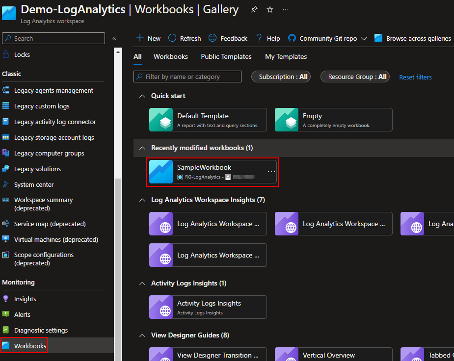
First, head to Workbooks on the left and then choose the Quick Start, Empty option.

You will be presented with an entirely blank workbook. Go ahead and hit the Add option (right under the Owl icon) and choose Parameters.

Then choose Add again (it’s now under the Parameters box) and choose Query. You should then have something that looks like this, a blank parameter and query.

Parameters are how we add dynamic fields to our queries. Go ahead and hit Add Parameter and configure it as shown below.

The Parameter Name is how we actually refer to the parameter in the queries. Don’t put a space in it. The display name is how it will show in the workbook, and the information is what you will see if you hover over the information bubble. While you can configure the time range options however you like, there is obviously no point in offering 90 days if you only have a 30-day retention period.

Once you have it filled out, just hit Save at the top.

Then, add a second Paramter like this. Once configured, hit Save.

Then, hit Done Editing, on the bottom of the Query Configuration.

This will reduce it to the same way it would present in the non-editing view of the workbook (See below). If you need to edit it again, hit the edit button just below them and way off to the right.

Next, into the query writer, drop this in.

SampleCollection_CL
| where TimeGenerated{TimeRange}
| summarize arg_max(TimeGenerated,*) by ComputerName
| extend ComputerUpTimeNegative = toint(ComputerUpTime) * -1
| extend LastBoot = datetime_add('day',(ComputerUpTimeNegative),now())
| summarize count() by bin(todatetime(LastBoot), 1d)
| sort by LastBoot
| render barchart

You will need to make sure to set a Time Range in the parameter you just made, and make sure that the Time Range setting and Visualization setting are set to Set By Query.

Now the Time Range at the top is controlling how far back in ingested data we are looking. In other words, if you want to see data for any device that has checked in (has a time generated date of X or greater) in the past 14 days, set the time range to 14 days.

Depending on how much data you have, you will get something like this as a graphed out result.

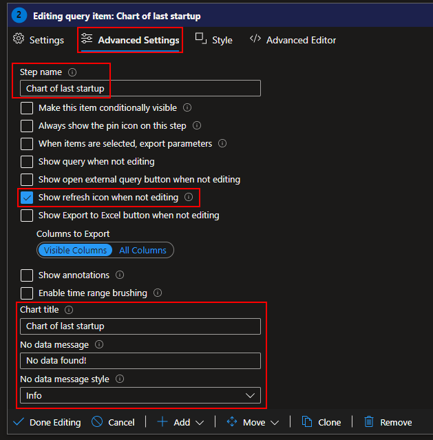
If you change to the Advanced Settings tab of the query (see below), you will find some options to configure the query items like its name and the ability to refresh it.

Note: There is likely little value in enabling export of this as it would just give you the graph itself, not the data behind the graph.

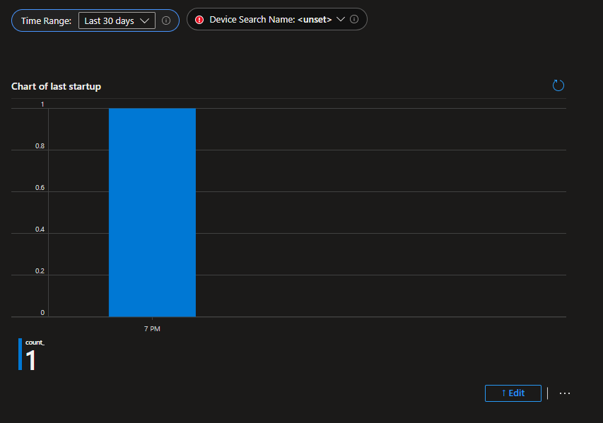
If you change to the Style tab, you will find options to adjust its size. I will be changing it to 50% width.

If you hit done editing, you will see how this looks in its final non-editing view minus the continued presence of an edit button. Obviously, I don’t have the same volume of data here as in some of my other screenshots.

Next, repeat that same process. Add a query, fill in the options for the name, size it to 50%, and fill in the below query. You will want to adjust the Advanced Settings to allow export on this one.

Note: If you want, you can actually just hit Edit on the existing query and use the Clone option at the bottom of it to quickly duplicate it.

SampleCollection_CL
| summarize arg_max(TimeGenerated,*) by ComputerName
| where isnotempty( ComputerName)
| extend ComputerUpTimeNegative = toint(ComputerUpTime) * -1
| extend LastBoot = datetime_add('day',(ComputerUpTimeNegative),now())
| project TimeGenerated, LastBoot, ComputerName, SerialNumber, Model
| sort by LastBoot asc

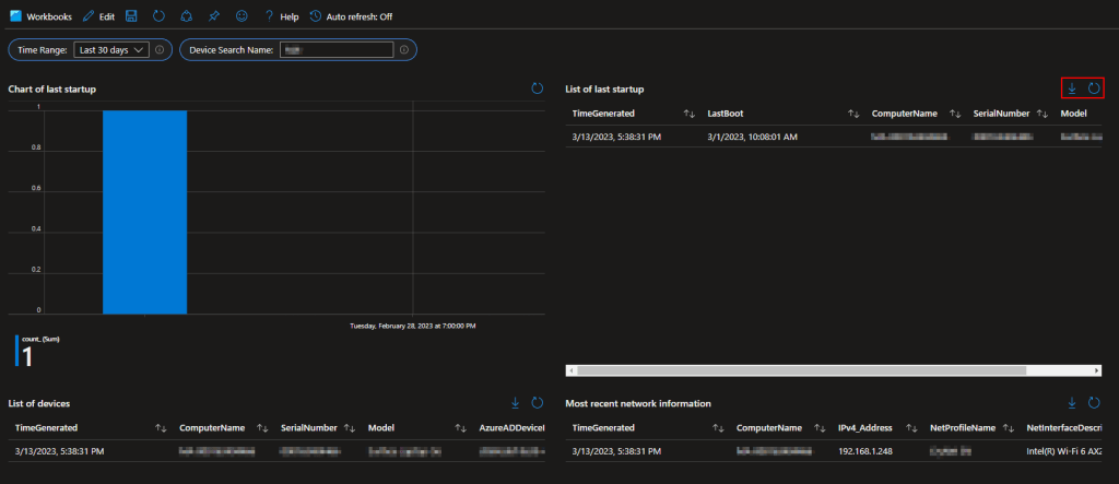
The result (once you hit Done Editing) should look like this. Now we have our graph on the left, and the exportable raw data behind that graph on the right.

Next, shocker, add another query and drop this in. Again, you can just use the clone option and alter the name. Again, make this one exportable.

SampleCollection_CL
| where TimeGenerated{TimeRange}
| summarize arg_max(TimeGenerated,*) by ComputerName
| project TimeGenerated, ComputerName, SerialNumber, Model, AzureADDeviceID, ManagedDeviceID, ManagedDeviceName

And again, add another query. Again, clone it, rename it, etc. Make it exportable.

SampleCollection_CL
| where TimeGenerated{TimeRange}
| where ComputerName contains "{DeviceSearchName}"
| summarize arg_max(TimeGenerated, *) by ComputerName
| extend NetworkAdapters_Expanded = todynamic(NetworkAdapters)
| mv-expand NetworkAdapters_Expanded
| evaluate bag_unpack(NetworkAdapters_Expanded )
| extend IPv4_Address = NetIPv4Adress 
| project TimeGenerated, ComputerName, IPv4_Address, NetProfileName, NetInterfaceDescription

You will need to start typing something into the Computer Name parameter to get the last query to run.

In the end, you should have something that looks like this.

Note that all (applicable) queries have a refresh option and an export option. When it comes to Workbooks, queries do have a 250-line limit for how many lines they show as a result but, exporting it exports the full data including beyond the first 250 lines.

Lastly, you can hit the save icon and save the new workbook. You may need to hit Done Editing to see this option. You will need to give it a name as well as location to store the workbook. This is actually its own Azure object just like the workspace itself, or the Function App.

It may then be a few minutes but eventually your new workbook will appear in the workbook menu for others to access and get data from. The workbooks do save whatever value was last entered into the parameters when save was last hit.

Importing the Workbook JSON:

You can find the JSON for the workbook above here. You will need to make a new workbook, head to the JSON view (</>), and paste the JSON in. Then choose Apply in the top right. You will then still need to save the workbook.

This does assume you named your tables and values the same as mine. If not, you can either edit them manually in the JSON (CTRL+F and replace “SampleCollection_CL”) or, save the workbook and then go into edit view to alter them.

Conclusion:

You should now have some knowledge on how queries are written, how workbooks are made, and what value you can provide with even some very basic data.

The Next Steps:

See the index page for all new updates!

Log Analytics Index – Getting the Most Out of Azure (azuretothemax.net)

Disclaimer

The following is the disclaimer that applies to all scripts, functions, one-liners, setup examples, documentation, etc. This disclaimer supersedes any disclaimer included in any script, function, one-liner, article, post, etc.

You running this script/function or following the setup example(s) means you will not blame the author(s) if this breaks your stuff. This script/function/setup-example is provided AS IS without warranty of any kind. Author(s) disclaim all implied warranties including, without limitation, any implied warranties of merchantability or of fitness for a particular purpose. The entire risk arising out of the use or performance of the sample scripts and documentation remains with you. In no event shall author(s) be held liable for any damages whatsoever (including, without limitation, damages for loss of business profits, business interruption, loss of business information, or other pecuniary loss) arising out of the use of or inability to use the script or documentation. Neither this script/function/example/documentation, nor any part of it other than those parts that are explicitly copied from others, may be republished without author(s) express written permission. Author(s) retain the right to alter this disclaimer at any time. 

It is entirely up to you and/or your business to understand and evaluate the full direct and indirect consequences of using one of these examples or following this documentation.

The latest version of this disclaimer can be found at: https://azuretothemax.net/disclaimer/